Consumer Reactions to Armed Conflicts: Sunday Special Edition of Macro Monday … Duration is Key Across Variables
- US armed conflict started over the last 48 hours.
- We examine the prior 5 armed conflicts for patterns of consumer and market reactions.
- We add this analysis to our weekly Macro Monday analysis of US consumer activity through last week.
On Friday evening 2/27 President Trump announced “major combat operations” in a video release. At roughly 1 am ET on Saturday, 2/28, missile strikes on Iran commenced. We keep in mind 70% of the US economy is consumer, and consumers do tend to have a pattern of reaction to conflicts. We have added an analysis & summary of such impacts, including Sentiment, other consumer macro variables, and consumer subsector performance as seen during armed conflicts since WWII. In each case, the duration of conflict is a key variable. Consumers will do what they have always done, passively assess how long this conflict may last and how it will impact their lives (economic strength, fuel prices, jobs, interest rates).
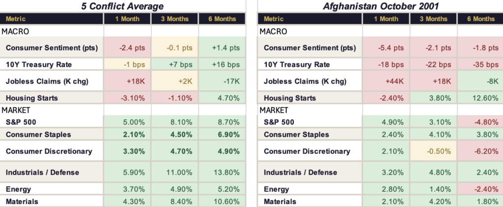
We analyzed consumer macro and market reactions to 5 conflicts since WWII: Korea (1950 start), Vietnam (1964 start), Gulf War (1991), Afghanistan (2001), and Iraq (2003). There were, of course, vastly different speeds and frequencies of market information and economic data across those 53 years. The anchor date, slope, intensity, and duration of each conflict were very different. We think Afghanistan 2001 could be the best proxy (as of now) for current events – a conflict that is modern but doesn’t end quickly. We include the average impacts and 2001 impacts in the table below.
We particularly highlight consumer staples. As Afghanistan wasn’t resolved quickly and involved more boots on the ground and US involvement, staples outperformed more and more over time. Jonathan Feeney adds, “This time around, the defensive staples trade is compounded by their relative AI resilience. In places like protein (HRL, JBS), there’s all that plus an undemanding valuation and positive fundamental inflection … there are some incredible opportunities.”
Sources: Optimal Advisory Analysis, University of Michigan Survey of Consumers, FRED STL, Bloomberg
Stocks will move, but the important gas price discussion will also ramp up quickly this week as oil moves, given Iran’s role in the energy sector and potential related blockades. Sunday early futures are suggesting a 10% move in crude prices, and some discussions about $100 bbl oil are starting, which would be a further 25% increase. The math works out such that a good rule of thumb is that the middle 60% of consumers are impacted by gas prices. They feel a headwind or tailwind of about 50 bp per 10% y/y of fuel price change. If gasoline prices were to jump 10-30% y/y, we’d expect most consumers feel a headwind or “tax” of 50-150 bp in spending. As seen below, consumer velocity is running about +150 bp y/y by our math, so a fuel impact would be felt and therefore impact other spending. Of course, fuel costs eventually can hit COGS through product and shipping costs, too. These impacts are felt across consumer. The duration of all these impacts from geopolitical events is what will matter most.
Last Week:
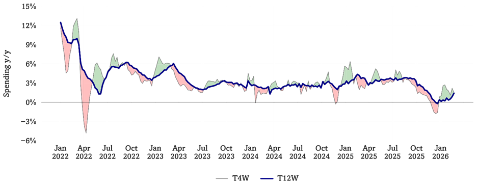
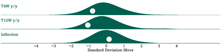
Our Consumer Velocity tracker remained at positive but muted, running up +1.5% y/y. This metric was running -1.6% y/y in mid-December but was up +3-4% in 3Q25. Our analysis of the trailing 4-week moving average of sales at 133 retailers and consumer concepts is running up +1.5% y/y (0.8 standard deviations below average since the start of 2022). The trailing Consumer Velo 12-week trend is up +1.4% y/y, its highest level since mid-November (1.0 standard deviations below average) vs. +0.8% y/y last week, leading to a shorter vs. longer-term inflection of +0.1% (0.2 standard deviations above average). See Fig 1-2.
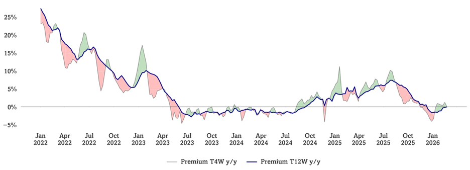
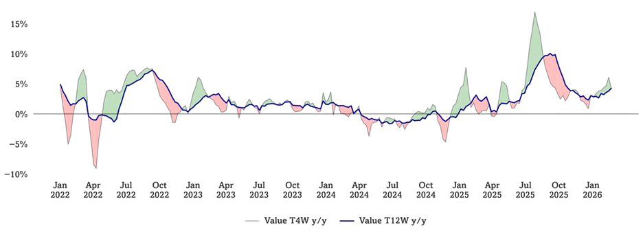
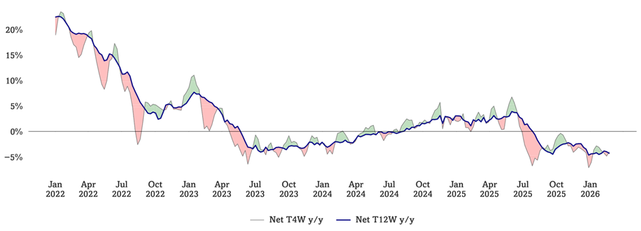
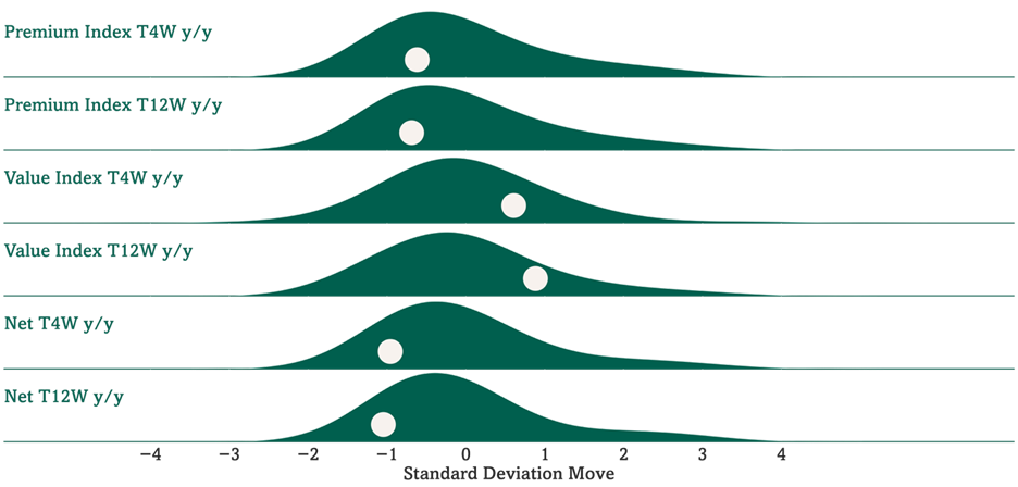
We note moderating spend at both our Value & Premium indices and Value continues to outpace. This is particularly interesting in early 2026 with white collar unemployment increasing and our AIR (AI-Resistant) names from Consumer Staples. We use a combination of consumer spending and psychographic monitoring to track “trade up” and “trade down” trends. Optimal’s premium monitor is running up +0.1% y/y on a T4W basis and flat y/y on a T12W basis, running 400 bp (0.9 standard deviations below average) and 430 bp (1.1 standard deviations below average) respectively below our Value Monitor, which is running up +4.2% y/y on a T4W basis and up +4.3% y/y on a T12W basis. See Fig 3-6.
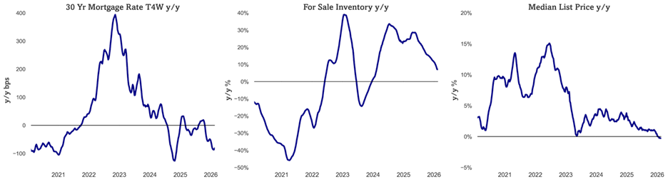
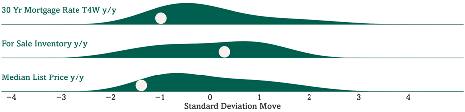
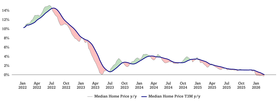
US 30Y FRM dropped below 6% for the first time in over 3 years. US 30Y FRM rate continues to run down, now running down -81 bps y/y on a T4W basis (1.0 standard deviations below average since 2020) and at only 5.98% for the most recent week. MBA’s mortgage applications for purchase continue to run up +9% y/y while refinance applications running up +132% (a low base, but a necessary step to create eventual velocity). Median home prices are flat y/y (-1.3 standard deviations below average since 2020). Roughly 18% of Americans sell, build, fix, lend to, and furnish homes – velocity matters for the economy. See Fig 7-10.
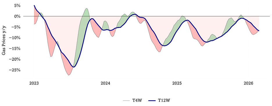
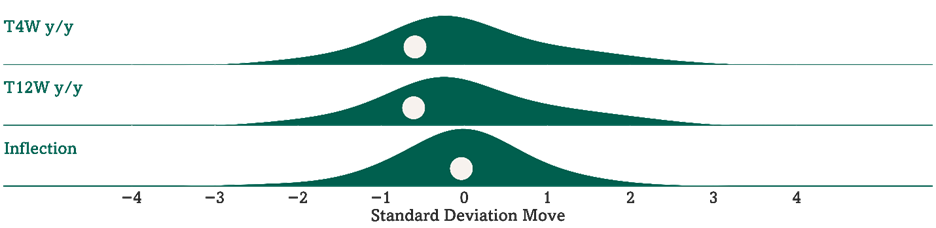
Gasoline prices continued meaningful y/y declines, with the effects of the Iran conflict still on the come. Gas prices ran down -6.8% y/y on a T4W basis and on a T12W y/y basis, corresponding to a -0.1% inflection between shorter- and longer-term trends (flat relative to average). We have had lots of recent conversations on oil and fuel prices due to developments in Venezuela, and military activity in Iran complicates the calculus further. Traffic through the Strait of Hormuz has reportedly already slowed substantially, which could significantly increase crude oil prices if Iran makes the Strait unsafe for commercial traffic. OPEC Plus has already pledged to increase oil production by 206,000 barrels / day in April to attempt to offset the impact of oil price disruptions, but oil prices are still generally expected to rise once trading resumes. Meanwhile, markets are still mixed on the Venezuela action. Generally, lower-income consumers spend about 5% of their total spend on fuel, and higher-income consumers spend about 2.5% – so a 10% move in gas prices drives 25-50 bp headwind or tailwind. Utilities (electricity and heating fuel) run from about 9% of lower-income household spending to 4% for higher-income households. Duration of change matters – eventually causing Consumer Sentiment shifts, which then drive more or less discretionary spending. On the cost side, Feeney noted last week that the Optimal Cost Factor continues to work lower, down -12.6% y/y. Broad-based commodity price declines have pushed many measured ticker & sector cost indices lower. See Fig 11-12.
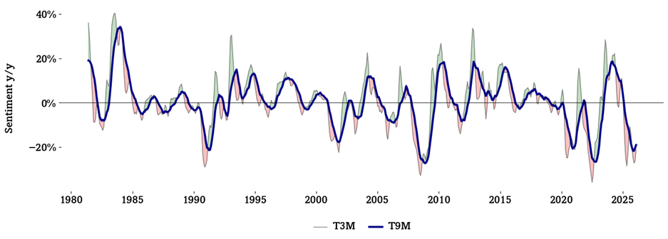
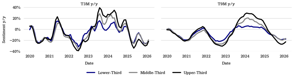
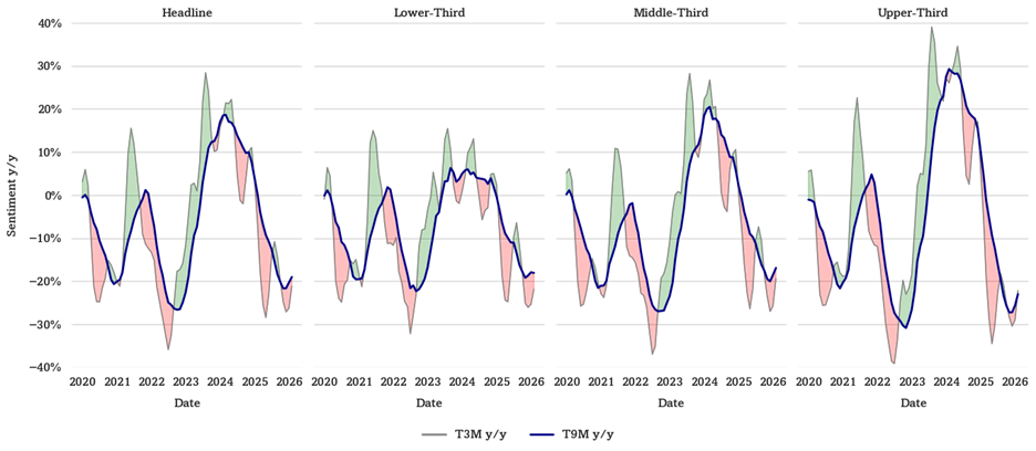
Rate of change is less bad for Consumer Sentiment as it is now down -21% y/y over the past three months, but is only down -13% y/y in February for all respondents -9% for higher-income respondents. Overall, headline Sentiment has declined -21% y/y on a T3M basis (1.7 standard deviations below average) and -19% y/y on a T9M basis (1.8 standard deviations below average). This compares to -20% y/y on a T9M basis last month, marking the third month since late 2024 and fourth month since early 2024 where longer-term Sentiment y/y did not decrease from the prior month. Upper-third income Sentiment has declined -22% y/y on a T3M basis (1.6 standard deviations below average), after declining -29% y/y T3M last month. Middle-income Sentiment has declined -19% y/y on a T3M basis (1.5 standard deviations below average) compared to -26% last month, and lower-income Sentiment has declined -22% y/y on a T3M basis (1.9 standard deviations below average) compared to -25% last month. See Fig 13-16.
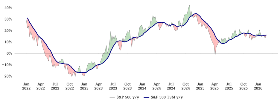
Consumer Wealth Effect Index still below historical average. Optimal Advisory’s Wealth Effect Index is at 8.8% y/y (0.1 standard deviations below average since the start of 2022). This metric was running +15.4% y/y in October 2025. With home prices flat y/y and crypto returns sharply down in recent weeks we note the “flywheel” of wealth effect is more muted. See Fig 17-20.
Multifactor Macro Market Model suggestive of softness, rebound. Optimal’s Multifactor Macro Market Model projects the S&P 500 as well as bull and bear cases based on lagged data for 12 macroeconomic factors. The model suggests the S&P 500 to fall to just below 6000 by next March, before rebounding back up to 6400 by May. We use this model as a guide to how macro would guide the market, given our analysis of current variables. This is, of course, outside of other factors at work. See Fig 21-22.
Additional Upcoming Optimal Virtual Meetings
Trade Up, Tariffs & Changing Tastes: 2026 Outlook From The Front Lines of U.S. Premium Alcohol – March 6th @ 11AM ET
Hosted by: Jonathan Feeney – Managing Partner & Co-Founder
Globally Distributed AI Infrastructure and what it means for Agentic Commerce, AI Devices, and Experiences – March 13th @ 11AM ET
Hosted by: David Schick – Managing Partner & Co-Founder
Sports & Sports Betting Ecosystems with Danny Funt – March 20th @ 11AM ET
Hosted by: David Schick, Jonathan Feeney, & David Katzman – Vice President
Figures 1-2: Optimal Advisory Consumer Velocity Monitor
Source: Optimal Advisory Analysis, Bloomberg Second Measure
Consumer Spending y/y Relative to Historical Average
Source: Optimal Advisory Analysis, Bloomberg Second Measure
Figures 3-6: Optimal Advisory Premium vs Value Monitor
Source: Optimal Advisory Analysis, Bloomberg Second Measure, Google Trends
Optimal Advisory Premium vs Value Indices Relative to Historical Averages
Source: Optimal Advisory Analysis, Bloomberg Second Measure, Google Trends
Figures 7-10: Housing Kinetic Energy
Source: Optimal Advisory Analysis, Freddie Mac, Zillow, Redfin
Mortgage Rates, For Sale Inventory, & Median List Price y/y Relative to Historical Averages (Since 2020)
Source: Optimal Advisory Analysis, Freddie Mac, Zillow, Redfin
Figures 11-12: Gas Prices y/y
Source: Optimal Advisory Analysis, U.S. Energy Information Administration
Gas Prices y/y Relative to Historical Averages (Since 1992)
Source: Optimal Advisory Analysis, U.S. Energy Information Administration
Figures 13-16: Consumer Sentiment T3M and T9M y/y
Source: Optimal Advisory Analysis, University of Michigan Consumer Survey
Sentiment y/y by Income Tercile Relative to Historical Averages
Source: Optimal Advisory Analysis, University of Michigan Consumer Survey
Comparison of Sentiment y/y Across Income Terciles
Source: Optimal Advisory Analysis, University of Michigan Consumer Survey
Figures 17-20: Consumer Wealth Effect & Components y/y
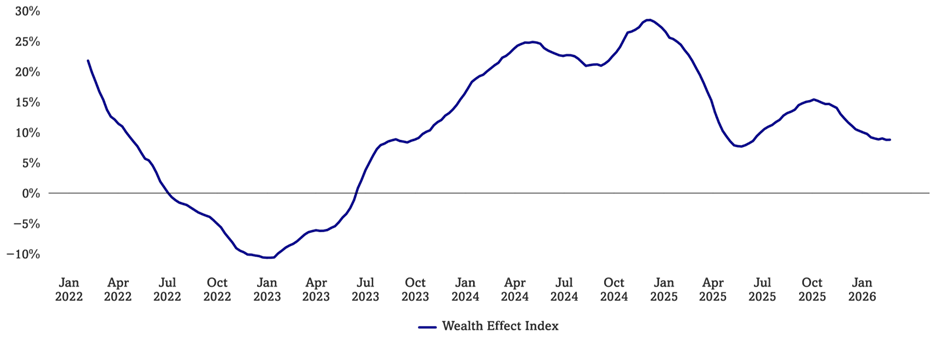
Source: Optimal Advisory Analysis, Bloomberg, Zillow, Redfin
Median Home Price y/y, S&P 500 y/y, & Wealth Effect Index (Since 2022)
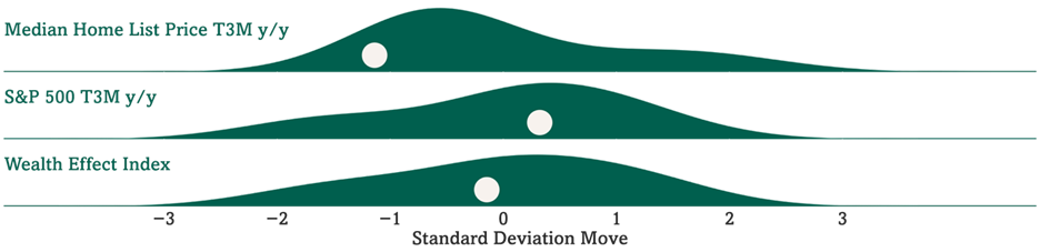
Source: Optimal Advisory Analysis, Bloomberg, Zillow, Redfin
Figures 21-22: Optimal Advisory Multifactor Macro Market Model
Historical Test Predictions vs. Actual (On Test Data Only)
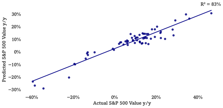
Source: Optimal Advisory Proprietary Analysis, Bloomberg, FRED, BLS, BEA, OECD, University of Michigan Consumer Sentiment Survey, U.S. Census Bureau, FRB
Actual & Projected S&P 500 (Including Training & Test Data) with Confidence Intervals
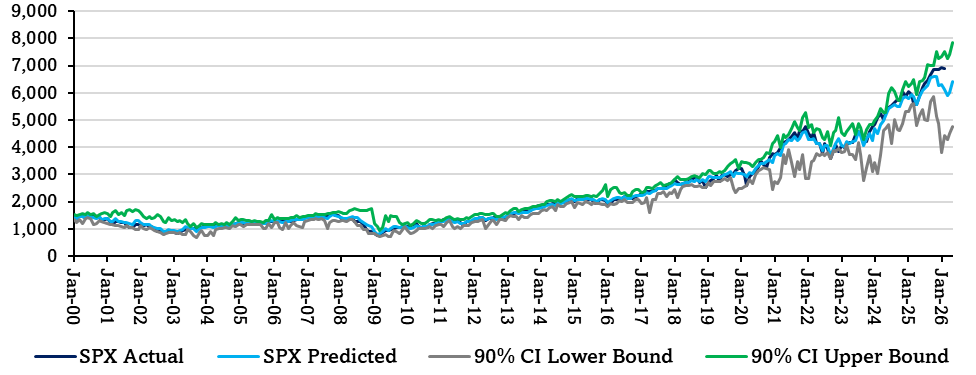
Source: Optimal Advisory Proprietary Analysis, Bloomberg, FRED, BLS, BEA, OECD, University of Michigan Consumer Sentiment Survey, U.S. Census Bureau, FRB
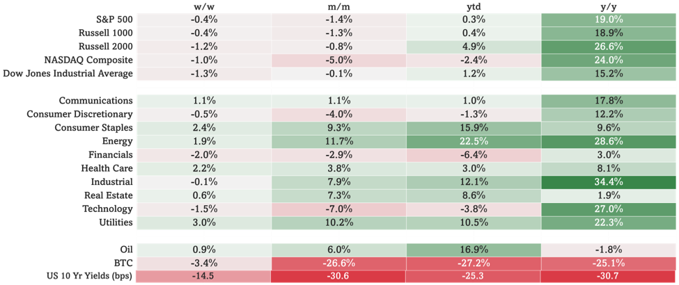
Figure 23: Index & Sector Performance
Source: Optimal Advisory Analysis, Bloomberg, prices at market close 2/27/2026