More Gas Price Math – When Behavior Changes; Premium Spend is Tracking Weaker than Value; Unemployment Rate Less Accurate than Prior Periods: Macro Monday

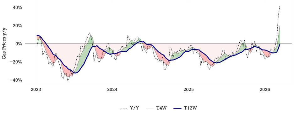
By David Schick and Jonathan Feeney and David Katzman and Jack Hermann Published on March 16, 2026 PDF

1 – Magnitude and duration of gas price moves matter. Now at 40% y/y inflation we’d expect trip consolidation and about 200 bp discrectionary headwind (or most of the current spending pace) if pressure persist another 4-6 weeks.

2 – Our analysis shows Value spend with significantly more momentum than Premium spend.

3 – Unemployment % is not a metric we think is useful in the 2020s, see Premium v Value discussion below as to why.

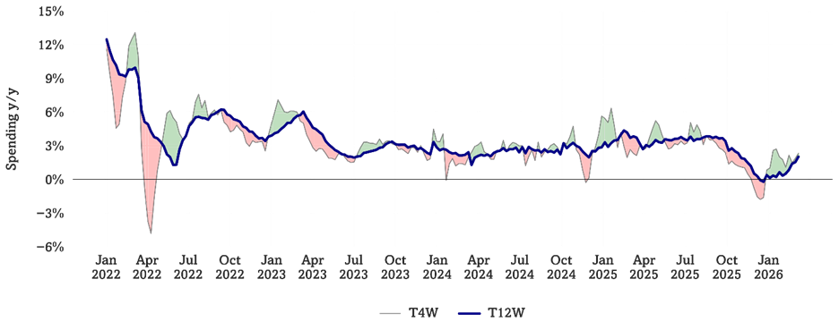
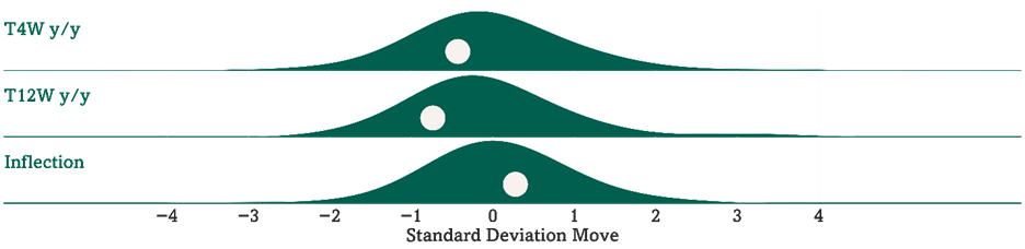
So far, consumer activity hasn’t moved much yet … our tracker is fairly stable – but the trend is still softer than 3Q25. Our Consumer Velocity tracker remained positive but muted, running up +2.3% y/y T4W. This metric was running -1.6% y/y in mid-December but was up +3-4% in 3Q25. Our analysis of the trailing 4-week moving average of sales at 133 retailers and consumer concepts is running up +2.3% y/y (0.4 standard deviations below average since the start of 2022). The trailing Consumer Velo 12-week trend is up +2.0% y/y (0.7 standard deviations below average) vs. +1.5% y/y the prior week, leading to a shorter vs. longer-term inflection of +0.3% (0.3 standard deviations above average). See Fig 1-2.

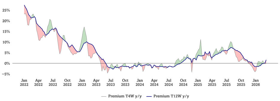
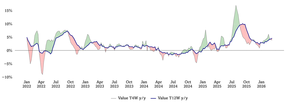
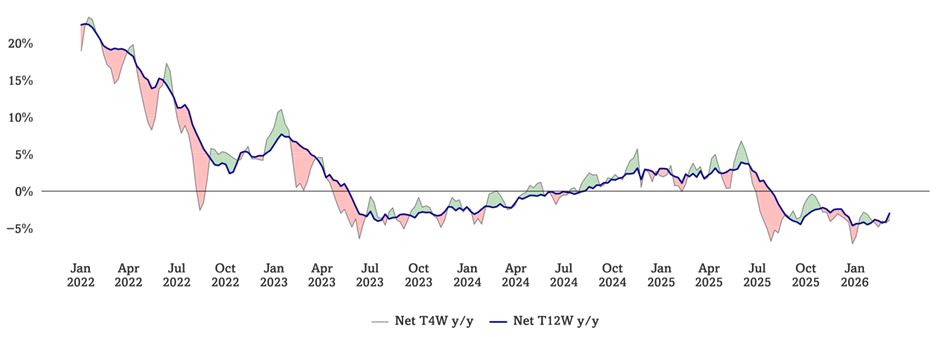
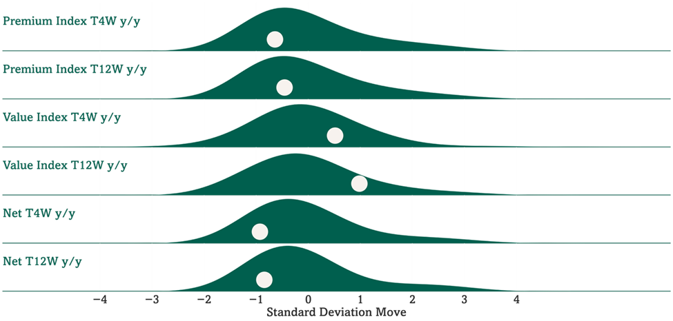
Trade away from Premium into Value (and why Unemployment Rate is not as accurate a signal as it once was, to us). We use a combination of consumer spending and psychographic monitoring to track “trade up” and “trade down” trends. Optimal’s premium monitor is running flat y/y on a T4W basis and +1.6% y/y on a T12W basis, running 450 bp (0.9 standard deviations below average) and 390 bp (0.8 standard deviations below average) respectively below our Value Monitor, which is running up +4.8% y/y on a T4W basis and up +4.5% y/y on a T12W basis. We have had many client conversations about unemployment rate versus the softness our tracking metrics began to show in 4Q25 and the continued muted pace and migration to Value from Premium. See Fig 3-6. The current “Unemployment Rate” in the mid 4% range is slightly higher than the last few years and fairly flat to 2017. How, then, can we live in a consumption economy and have lots of variability to spending? The official, stated rate measures Americans filing for unemployment as a percentage of the total labor force. But today, less frictional tech platforms and marketplaces exist for unemployed and underemployed to seek income (drive an Uber, deliver Door Dash, online contract work). So we expect that filing unemployment claims is likely not the primary step or solution for workers. Instead, we keep our eye on aggregate spend, job listings, and JOLT data.

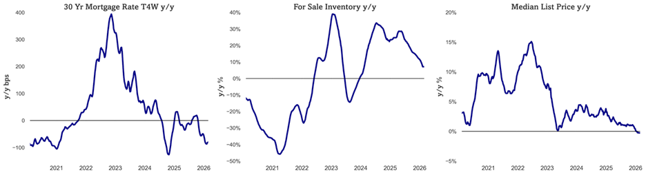
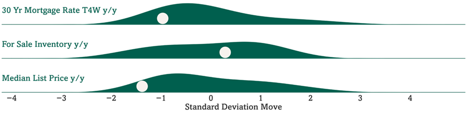
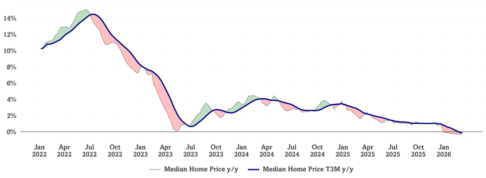
Housing potential & kinetic energy is more muted as mortgage rates pressured higher by oil inflation. US 30Y FRM rate continues to run down y/y, now running down -76 bps y/y on a T4W basis (0.9 standard deviations below average since 2020). MBA’s mortgage applications for purchase continue to run up +8% y/y while refinance applications running up +81% (a low base, but a necessary step to create eventual velocity). Median home prices are flat y/y (-1.3 standard deviations below average since 2020). Roughly 18% of Americans sell, build, fix, lend to, and furnish homes – velocity matters for the economy. See Fig 7-10.

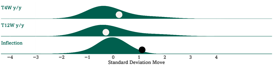
Gasoline inflation is now +41.5% y/y for the week ending last Friday following +30.3% the week prior. Gas prices ran up +19.5% y/y on a T4W basis and down -1.1% y/y on a T12W basis, corresponding to +20.6% inflection between shorter- and longer-term trends (1.1 standard deviations above average since 2017, which includes 2021 spikes, and 3.1 standard deviations above average since 2023). It is worth noting US discretionary consumer comp store sales broadly decelerated only after gas y/y prices were +30% in the fall of 2007. Our analysis of, and experience with, prior slowdowns driven by external macro stimuli suggests gas price inflation of 30%+ y/y begins to impact discretionary spending after about 6-8 weeks. Generally, lower-income consumers spend about 5% of their total spend on fuel, and higher-income consumers spend about 2.5% – so a 10% move in gas prices drives 25-50 bp headwind or tailwind. Utilities (electricity and heating fuel) run from about 9% of lower-income household spending to 4% for higher-income households. Duration of change matters – eventually causing Consumer Sentiment shifts, which then drive more or less discretionary spending. On the cost side, Jon Feeney noted last week that the Optimal Cost Factor continues to work lower, down -9.2% y/y. Higher energy & oil prices moving input costs index higher, but still down significantly y/y. See Fig 11-12.

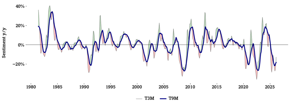
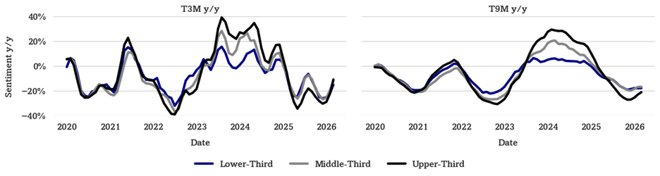
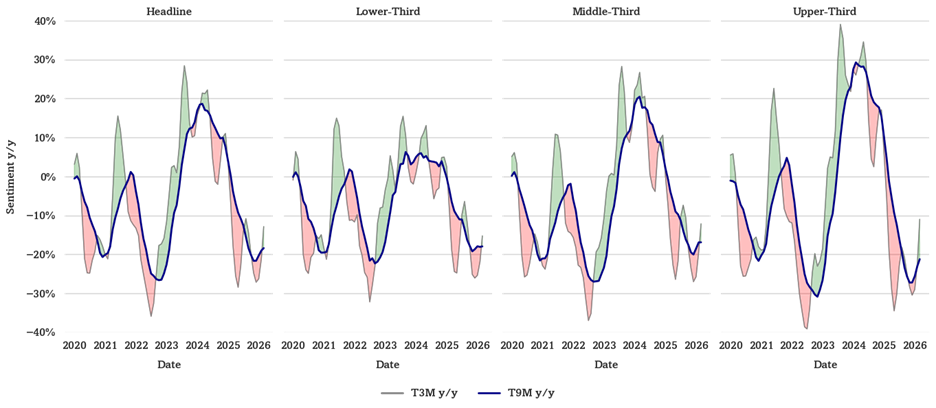
Sentiment is very weak (right at GFC lows!) but is now lapping very weak comparisons. Overall, headline Sentiment is down -2.5% y/y and -13% y/y on a T3M basis (1.1 standard deviations below average) and -18% y/y on a T9M basis (1.8 standard deviations below average). This compares to -13% y/y on a T9M basis last month, marking the third consecutive month where longer-term Sentiment y/y improved from the prior month. Upper-third income Sentiment has declined -11% y/y on a T3M basis (0.8 standard deviations below average), after declining -22% y/y T3M last month. Middle-income Sentiment has declined -12% y/y on a T3M basis (1.0 standard deviations below average) compared to -19% last month, and lower-income Sentiment has declined -15% y/y on a T3M basis (1.3 standard deviations below average) compared to -22% last month. See Fig 13-16.

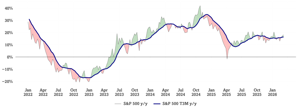
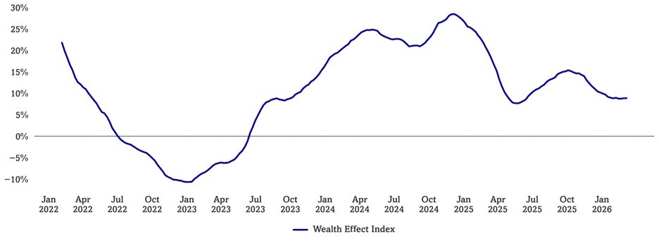
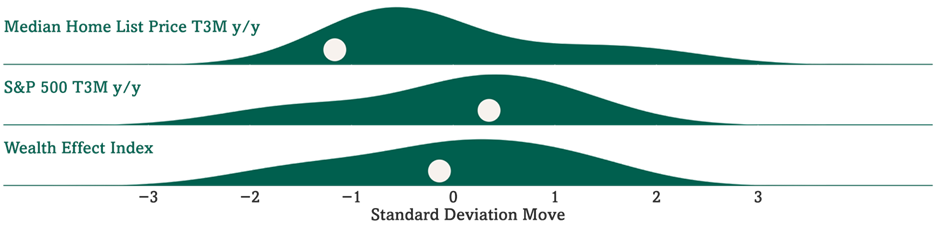
Consumer Wealth Effect Index is 600 bp below 3Q25 levels – a drag on Premium mindset. Optimal Advisory’s Wealth Effect Index is at 8.9% y/y (0.1 standard deviations below average since the start of 2022). This metric was running +15.4% y/y in October 2025. With home prices flat y/y and equity returns moving lower in recent days we note the “flywheel” of wealth effect is more muted. See Fig 17-20.

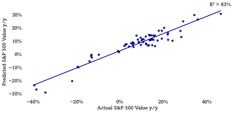
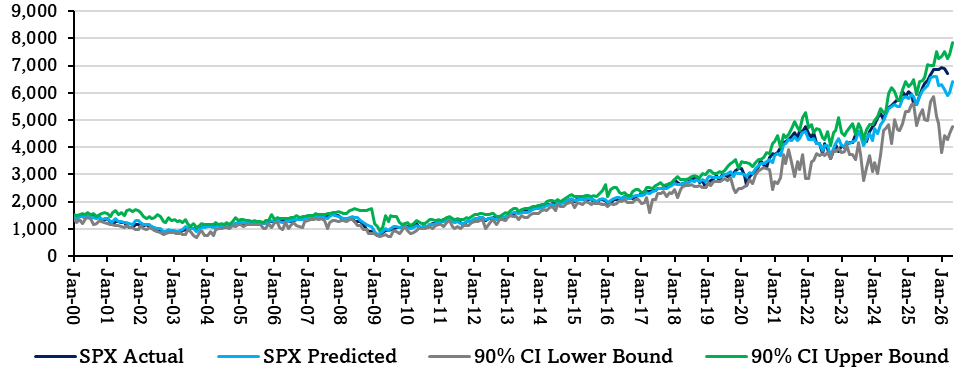
Multifactor Macro Market Model has been suggestive of March 2026 softness, rebound. Optimal’s Multifactor Macro Market Model projects the S&P 500 as well as bull and bear cases based on lagged data for 12 macroeconomic factors. The model has suggested the S&P 500 to fall to just below 6000 by this month, before rebounding back up to 6400 by May. We use this model as a guide to how macro would guide the market, given our analysis of current variables. This is, of course, outside of other factors at work. See Fig 21-22.

Upcoming Optimal Virtual Meetings

Sports & Sports Betting Ecosystems with Danny Funt
March 20th @ 11AM ET
Hosted by: David Schick, Jonathan Feeney, & David Katzman – Vice President
Click to Register

Figures 1-2: Optimal Advisory Consumer Velocity Monitor

Source: Optimal Advisory Analysis, Bloomberg Second Measure

Consumer Spending y/y Relative to Historical Average

Source: Optimal Advisory Analysis, Bloomberg Second Measure

Figures 3-6: Optimal Advisory Premium vs Value Monitor

Source: Optimal Advisory Analysis, Bloomberg Second Measure, Google Trends

Optimal Advisory Premium vs Value Indices Relative to Historical Averages

Source: Optimal Advisory Analysis, Bloomberg Second Measure, Google Trends

Figures 7-10: Housing Kinetic Energy

Source: Optimal Advisory Analysis, Freddie Mac, Zillow, Redfin

Mortgage Rates, For Sale Inventory, & Median List Price y/y Relative to Historical Averages (Since 2020)

Source: Optimal Advisory Analysis, Freddie Mac, Zillow, Redfin

Figures 11-12: Gas Prices y/y

Source: Optimal Advisory Analysis, Bloomberg

Gas Prices y/y Relative to Historical Averages (Since 1992)

Source: Optimal Advisory Analysis, Bloomberg

Figures 13-16: Consumer Sentiment T3M and T9M y/y

Source: Optimal Advisory Analysis, University of Michigan Consumer Survey

Sentiment y/y by Income Tercile Relative to Historical Averages

Source: Optimal Advisory Analysis, University of Michigan Consumer Survey

Comparison of Sentiment y/y Across Income Terciles

Source: Optimal Advisory Analysis, University of Michigan Consumer Survey

Figures 17-20: Consumer Wealth Effect & Components y/y

Source: Optimal Advisory Analysis, Bloomberg, Zillow, Redfin

Median Home Price y/y, S&P 500 y/y, & Wealth Effect Index (Since 2022)

Source: Optimal Advisory Analysis, Bloomberg, Zillow, Redfin

Figures 21-22: Optimal Advisory Multifactor Macro Market Model

Historical Test Predictions vs. Actual (On Test Data Only)

Source: Optimal Advisory Proprietary Analysis, Bloomberg, FRED, BLS, BEA, OECD, University of Michigan Consumer Sentiment Survey, U.S. Census Bureau, FRB

Actual & Projected S&P 500 (Including Training & Test Data) with Confidence Intervals

Source: Optimal Advisory Proprietary Analysis, Bloomberg, FRED, BLS, BEA, OECD, University of Michigan Consumer Sentiment Survey, U.S. Census Bureau, FRB

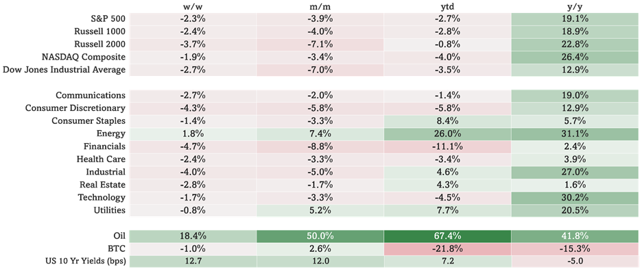
Figure 23: Index & Sector Performance

Source: Optimal Advisory Analysis, Bloomberg, prices at intraday 3/16/2026

DISCLOSURES AND DISCLAIMERS

Analyst Certification

The analyst primarily responsible for the preparation of this report attests to the following: (1) that the views and opinions rendered in this report reflect his or her personal views about the subject companies or issuers; and (2) that no part of the analyst’s compensation was, is, or will be directly related to the specific recommendations or views in this report.

Analyst Certifications And Independence

Each of the Optimal Advisory analysts whose names appear on the front page of this report hereby certify that all the views expressed in this Report accurately reflect our personal views about any and all of the subject securities or issuers and that no part of our compensation was, is, or will be, directly or indirectly, related to the specific recommendations or views of in this Report.

Optimal Advisory (the “Company”) is an independent equity advisory provider. The Company is not a member of the FINRA or the SIPC and is not a registered broker dealer or investment adviser. Optimal Advisory has no other regulated or unregulated business activities which conflict with its provision of independent advisory work.

Limitations Of Research And Information

This Report has been prepared for distribution to only qualified institutional or professional clients of Optimal Advisory. The contents of this Report represent the views, opinions, and analyses of its authors. The information contained herein does not constitute financial, legal, tax or any other advice. All third-party data presented herein were obtained from publicly available sources which are believed to be reliable; however, the Company makes no warranty, express or implied, concerning the accuracy or completeness of such information. In no event shall the Company be responsible or liable for the correctness of, or update to, any such material or for any damage or lost opportunities resulting from use of this data.

Nothing contained in this Report or any distribution by the Company should be construed as any offer to sell, or any solicitation of an offer to buy, any security or investment. Any research or other material received should not be construed as individualized investment advice. Investment decisions should be made as part of an overall portfolio strategy and you should consult with a professional financial advisor, legal and tax advisor prior to making any investment decision. Optimal Advisory shall not be liable for any direct or indirect, incidental or consequential loss or damage (including loss of profits, revenue or goodwill) arising from any investment decisions based on information or research obtained from Optimal Advisory.

Optimal Advisory may receive consulting or other compensation from securities mentioned but is not related to any recommendation in this report.

Reproduction And Distribution Strictly Prohibited

No user of this Report may reproduce, modify, copy, distribute, sell, resell, transmit, transfer, license, assign or publish the Report itself or any information contained therein. Notwithstanding the foregoing, clients with access to working models are permitted to alter or modify the information contained therein, provided that it is solely for such client’s own use. This Report is not intended to be available or distributed for any purpose that would be deemed unlawful or otherwise prohibited by any local, state, national or international laws or regulations or would otherwise subject the Company to registration or regulation of any kind within such jurisdiction.

Copyrights, Trademarks, Intellectual Property

Optimal Advisory, and any logos or marks included in this Report are proprietary materials. The use of such terms and logos and marks without the express written consent of Optimal Advisory is strictly prohibited. The copyright in the pages or in the screens of the Report, and in the information and material therein, is proprietary material owned by Optimal Advisory unless otherwise indicated. The unauthorized use of any material on this Report may violate numerous statutes, regulations and laws, including, but not limited to, copyright, trademark, trade secret or patent laws.

Additional Information is available upon request.

For more information on receiving Optimal Advisory, email: [email protected]